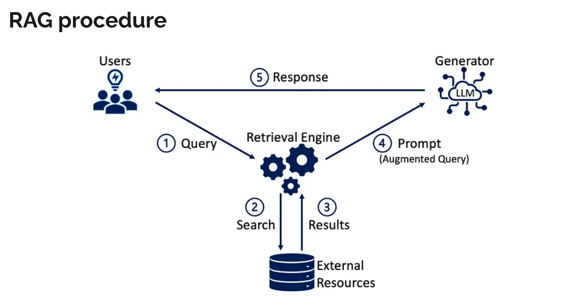
RAG @ CGU
We demonstrate the example usage of LangChain. Also in the labatory section, students are assigned to improve the embedding model.

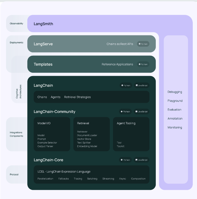
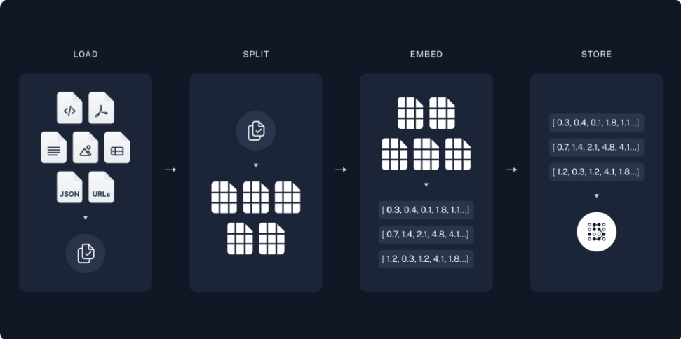
LangChain is an open-source framework designed to develop applications powered by language models. The framework is structured in layers (left image): LangChain-Core provides the fundamental building blocks, LangChain-Community offers integration components, and LangChain proper includes chains, agents, and retrieval strategies. LangServe enables deployment, while LangSmith provides observability. The right image illustrates the typical LangChain workflow through four key stages: LOAD (ingesting various document formats like PDFs, JSONs, and URLs), SPLIT (chunking documents into manageable segments), EMBED (converting text chunks into vector embeddings), and STORE (saving embeddings in vector stores for efficient retrieval). This pipeline enables applications to process, understand, and retrieve information from diverse data sources effectively. For more details, visit: LangChain GitHub Repository
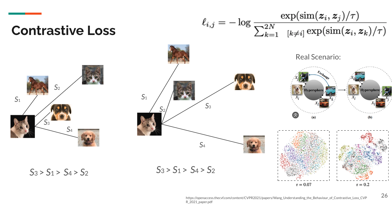
The embedding model plays crucial role when retrieving, an example of training the model is to leverage contrasive learning. Contrastive learning optimizes representations by minimizing the distance between similar pairs while maximizing it for dissimilar ones. The model implementation follows the approach presented in (Wang et al., 2021). The loss function ℓᵢⱼ shown at the top computes the negative log ratio between the similarity of positive pairs exp(sim(zᵢ, zⱼ)/τ) and the sum of similarities with all other samples in the batch. The temperature parameter τ controls the concentration of the distribution - lower values (e.g., τ=0.07) lead to more concentrated clusters as shown in the bottom right visualization, while higher values (e.g., τ=0.2) result in more spread-out embeddings. The model maps inputs into a hypersphere where semantically similar items are pulled closer together while pushing dissimilar ones apart.
